
Weibull analysis in maintenance fits a statistical life distribution to the operating times of a population of components, using both failures and units still running (suspensions), to estimate how the failure rate changes with age. Its shape parameter beta and characteristic life eta support inspection strategy, age replacement, spare planning and design comparison when the population is coherent.
Weibull is one of the quantitative tools of reliability engineering in maintenance, and uncertainty must accompany every parameter it produces. A sloped plot and values for beta and eta cannot close a decision on their own. Engineering needs to know which event ended life, where the clock started, which units remained in operation, which changes occurred, and whether the model represents the observations. A mixture of failure modes may form a persuasive graph while directing the wrong work.
Start with the decision question
Analysis begins with a bounded decision. For a bearing, the question may ask whether age replacement reduces economic risk. For a lining, it may estimate the probability of reaching the next outage. For a new component, it may compare two configurations under equivalent exposure.
The event must represent loss of function or a clearly defined life criterion. Opportunistic replacement, removal for inspection, and a unit still operating are not failures. They contribute information as right-censored observations. Discarding them overweights short lives and biases the estimate.
Parameters and physical interpretation
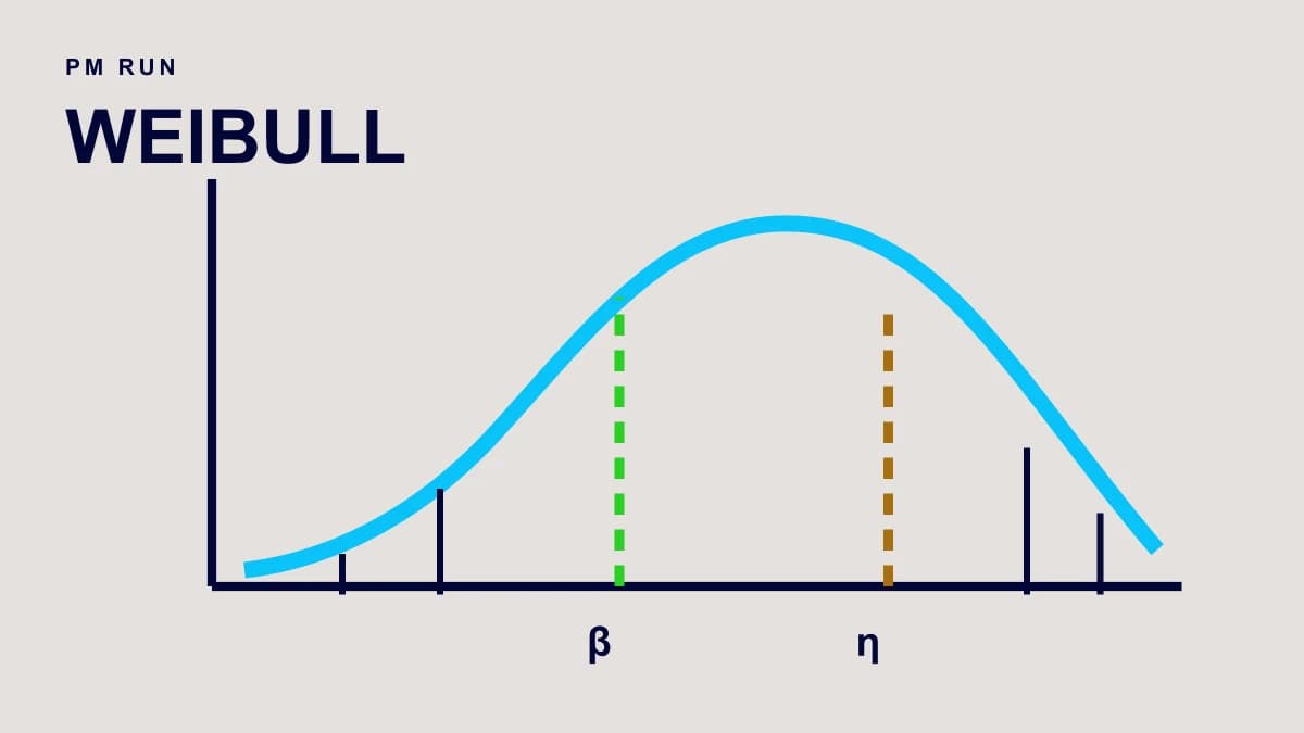
For a two-parameter Weibull, reliability at time t is R(t) = exp[-(t/eta)^beta]. Beta controls shape. Eta is characteristic life, where approximately 63.2% of the modeled population has failed. Eta is neither mean life nor an automatic replacement interval.
- Beta below 1: the fitted failure rate decreases, a pattern that can be compatible with early-life effects in some populations.
- Beta near 1: the rate is approximately constant and the model approaches an exponential distribution.
- Beta above 1: the fitted rate increases, potentially compatible with age-dependent mechanisms in a coherent population.
The three regimes correspond to the phases of the bathtub curve. These readings are clues rather than physical proof. A low beta may come from mixed lots, inconsistent installation, or an incorrect time origin. A high beta may reflect an administrative replacement limit instead of degradation. Asset evidence tests whether the statistical story makes engineering sense.
Construct a defensible population
The analysis unit should share design, service, load, environment, operating regime, and failure definition. A lubricant, seal, or work-procedure change can alter exposure and require a separate cohort. Repairable assets also require care because recurrent events are not independent new lives when repair does not restore an equivalent condition.
NIST distinguishes non-repairable populations from repairable systems. A lifetime Weibull models time to an event within a defined population. Recurrent processes in repairable systems may require intensity, trend, or recurrence models. The physical and maintenance process that generated the data should govern model choice.
Completed case: fan bearings
The plant operates 20 equivalent fans with the same drive-end bearing, continuous duty, and a similar load range. End of life was removal after confirmed bearing damage prevented operation inside internal vibration and temperature criteria.
Boundary and assumptions
| Field | Adopted definition |
|---|---|
| Life origin | return-to-service hour after a new bearing was installed |
| Failure endpoint | removal because confirmed bearing damage met the life criterion |
| Suspension | bearing still operating at the 9,000-hour data cut |
| Population | same part number, assembly method, lubricant, service, and speed range |
| Candidate model | two-parameter Weibull |
| Estimation | maximum likelihood with right censoring |
Failure times were 3,100, 3,650, 4,020, 4,380, 4,710, 5,180, 5,560, 6,030, 6,480, 7,010, 7,620, and 8,350 hours. Eight bearings remained in operation and were suspended at 9,000 hours. The review confirmed that no preventive replacements were hidden and every clock shared the same origin.
Worked calculation
The maximum-likelihood fit produced beta = 2.42 and eta = 9,051 hours after rounding. With R(t) = exp[-(t/9,051)^2.42], estimated reliability at 6,000 hours is 0.691. B10, when the model accumulates 10% failures, is approximately 3,575 hours. Estimated median life is 7,780 hours.
| Measure | Result | Proper use |
|---|---|---|
| Beta | 2.42 | indicates an increasing modeled rate within this population |
| Eta | 9,051 h | characteristic life, not a replacement rule |
| R(6,000) | 69.1% | modeled probability of surviving 6,000 h |
| B10 | 3,575 h | estimated quantile with sample uncertainty |
| Median | 7,780 h | 50% survival point under the model |
Model checking
The team did not accept the parameters simply because software converged. The probability plot was reviewed for curvature and influential observations. Residuals, log-likelihood, and alternative model comparisons were retained. Wide confidence intervals were expected because only 12 failures existed.
Two stratifications were explored. Four failures had documented contamination, and three occurred after an assembly revision. Records were not removed to improve straightness. Subsets were created only with a physical rationale, and the team concluded that the sample was still too small to claim separate parameter sets.
Decision from the fitted case
B10 did not become mandatory replacement at 3,575 hours. Such a policy would discard many functional bearings and could introduce assembly defects. The increasing rate justified closer attention after 3,000 hours, spare readiness for the likely window, and deeper investigation of contamination and installation mechanisms.
The route gained a targeted step after 3,000 hours with vibration, temperature, and seal-condition checks under comparable operation. At 6,000 hours, planning would review risk, outage opportunity, and evidence. Replacement remained conditional on condition, consequence, and the approved window unless a governing technical requirement said otherwise.
SAP PM plan, order, and history
Equipment history should preserve installation, position, counter, and replacement date. A removal order records the component's service hours, as-found condition, part number, confirmed mode, and return test. Units still operating enter the analysis extract as suspensions at the cut date rather than receiving fictitious failures.
The analysis produced a revised inspection plan, an hours-based strategy, and a confirmation task list. A condition notification opens when the route detects a deviation. The order executes the approved intervention. History preserves the connection among component, event, exposure, and evidence.
PM Run can distribute the route and work order, support scheduling, and return field confirmations to SAP PM under company configuration. Statistical fitting, mechanism interpretation, and replacement policy remain engineering responsibilities. The platform does not provide automatic Weibull diagnosis, sensors, or predictive AI.
Quantify uncertainty and test sensitivity
A point estimate hides width. Confidence intervals for beta, eta, and life quantiles should accompany the recommendation. B10 may be particularly uncertain with few failures. Planning needs the range rather than only the displayed decimal.
Sensitivity should also challenge the data boundary. A result that changes sharply after one date correction is fragile. A conclusion that depends on calling a preventive replacement a failure has a classification problem. Bootstrap or likelihood-profile methods can quantify uncertainty when the method and its assumptions are documented.
Data preparation controls
Before fitting, the analyst reconciles equipment hierarchy, component position, counter rollover, inactive periods, and event dates. Calendar time and operating hours answer different questions. Exposure that continued during standby would be incorrect for a component that was not rotating.
A data-quality table should show missing origins, unknown modes, repeated orders, changed part numbers, and units lost to follow-up. Each correction needs an audit trail. The original extract remains available so that a reviewer can reproduce the population.
Common application failures
- Removing surviving units and losing censoring information.
- Combining different components, functions, or failure modes.
- Using work-order dates instead of actual exposure.
- Turning eta into an optimal replacement interval.
- Treating beta as proof of a physical cause.
- Adding a location parameter without an engineering basis.
- Reporting forecasts without confidence intervals or model checks.
- Applying a simple lifetime model to a repairable-system recurrence process.
Indicators and learning window
The decision will be reviewed no later than 12 months and will also be brought forward if six new failures occur first. That maximum interval governs the decision review; a new statistical fit becomes eligible only when sample size, exposure, and data quality support estimation. Controls include counter completeness, correct suspension treatment, inspection compliance after 3,000 hours, failures before B10, recurrence by mode, and differences between predicted and observed survival.
The case target requires 98% of events with valid origin and exposure, no preventive replacement classified as failure, and 100% of removals with an as-found condition. A design or lubricant change opens a new cohort while preserving the previous series.
When Weibull fits the decision
Weibull models the life distribution of a population. MTTR and MTBF summarize event frequency and mean time under their own rules. Reliability engineering connects model, mechanism, consequence, and strategy. RCFA investigates events, while FMEA anticipates modes and effects.
Policy comparison for the fan bearings
The team compared three policies before changing the plan. The first retained uniform inspection across life. The second replaced every bearing at B10. The third intensified inspection after 3,000 hours and used condition for replacement. Each option was evaluated for intervention count, failure exposure, planned downtime, and assembly-induced risk.
B10 replacement created the lowest modeled exposure but would remove roughly 90% of units before the modeled event and multiply intrusive work. Uniform inspection ignored the increasing rate. Staged inspection focused capacity where risk increased while preserving serviceable components, provided the selected condition technique had demonstrated detection capability.
Uncertainty scenario
The review used a B10 range from 3,100 to 4,200 hours. Even at the lower bound, inspection beginning at 3,000 hours offered one opportunity before the uncertain region. A lower confidence bound below the first inspection, or failures without a detectable condition, would reopen the policy.
A second trigger was approved: two failures before 3,000 hours with the same mode require review of the cohort, assembly process, and Weibull assumption. The model must remain exposed to contradictory evidence.
Reproducible fitting package
The analysis package contains the source extract, inclusion rules, code version, starting values, convergence method, and unrounded output. Presentations use rounded figures, while the audit trail lets another analyst reproduce the fit.
A second reviewer checks five events against orders and counters. Corrected dates do not silently overwrite the extract. Every transformation receives a reason, owner, and date because each observation carries substantial weight in a small sample.
Admitting new events
New records are classified before joining the population. A contamination failure after a seal redesign may belong to a new cohort. A removal without confirmed damage remains censored. Monthly review monitors the queue, but parameters change only at the approved analysis window to avoid a policy oscillating with every record.
Decision record
The approved recommendation states the population, data cut, fitted model, uncertainty, rejected alternatives, owner, and review trigger. This record prevents a later team from treating B10 as an unconditional replacement rule. Any reuse for another bearing family requires a new applicability review.
Out-of-sample validation
The fan-bearing fit will be challenged against survival in the next cohort. The team defined expected ranges at 4,000, 6,000, and 8,000 hours before observing new outcomes. A material difference requires review of population, mode, and distribution rather than tuning the model to preserve the original conclusion.
Validation also compares failure order and suspension count. If the new cohort has less exposure, an absence of events will not be presented as proven improvement.
Communication for maintenance planning
The report translates probability into capacity and risk scenarios. It estimates how many components may enter the enhanced-inspection band, what spare demand could emerge, and when the decision will be reviewed. Decimal precision without an uncertainty range does not enter the schedule.
Technical references
- NIST/SEMATECH Engineering Statistics Handbook, Weibull, accessed August 23, 2026.
- NIST, repairable systems and non-repairable populations, accessed August 23, 2026.
- SAP Help Portal, Failure Data, accessed August 23, 2026.
To connect strategy, work orders, and field feedback to the corporate system, review PM Run's operational layer for SAP PM.
Frequently asked questions about Weibull analysis
What is Weibull analysis in maintenance?
It is the fit of a Weibull distribution to the life data of a coherent component population, counting failures and suspensions. Beta shows whether the failure rate falls, stays constant or rises with age, and eta gives the characteristic life. Maintenance uses the result to decide between inspection, condition monitoring and age-based replacement.
Can Weibull analysis forecast when to replace equipment?
It estimates the probability that a component survives to a given age, which is one input to replacement timing. The decision also needs the cost and consequence of failure against planned replacement, the uncertainty of the fit and whether a condition technique can detect degradation earlier. No model delivers a replacement date on its own.
Does beta above 1 prove wear?
It shows an increasing failure rate in the fitted model. A physical cause requires field evidence and sound stratification. Mixed populations can create the same pattern.
How should a unit that has not failed be handled?
Record its observed time as a suspension at the cut date. Maximum likelihood uses that information without declaring a failure.
When should the fit be repeated?
Repeat it after enough events, a design or operating change, removal of a common cause, or a material difference between predicted and observed results.